Loss Functions and Optimizers

When compiling your model you need to choose a loss function and an optimizer. The loss function is the quantity that will be minimized during training. The optimizer determines how the network will be updated based on the loss function.

Example compile step:

model.compile(optimizer='rmsprop', loss='binary_crossentropy', metrics=['accuracy'])

Loss Functions

There are some simple guidlines for choosing the correct loss function:

binary crossentropy (binary_crossentropy) is used when you have a two-class, or binary, classification problem.

categorical crossentropy (categorical_crossentropy) is used for a multi-class classification problem.

mean squared error (mean_squared_error) is used for a regression problem.

In general, crossentropy loss functions are best to use when the model you use is outputting probabilities.

Here is the Keras documentaiton for loss functions

Optimizers

There are many optimizers you can use and many are a variant of stochastic gradient descent. For all of them you will be able to tune the learning rate parameter. The learning rate parameter tells the optimizer how far to move the weights of the layer in the direction opposite of the gradient. This parameter is very important, if it is too high then the training of the model may never converge. If it is too low, then the training is more relibable but very slow. It is best to try out multiple different learning rates to find which one is best.

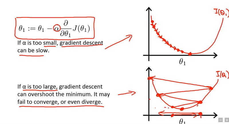
image source is this useful resource on learning rates

Here is the Keras documentation on optimizers.

Stochastic Gradient Descent

keras.optimizers.SGD(lr=0.01, momentum=0.0, decay=0.0, nesterov=False)

This is a common 'basic' optimizer and many optimizers are variants of this. It can be adjusted by changing the learning rate, momentum and decay.

• learning rate (lr)
• momentum - accelerates SGD in the relevant direction and dampens oscillations. Basically it helps SGD push past local optima, gaining faster convergence and less oscillation. A typical choice of momentum is between 0.5 to 0.9.
• decay - you can set a decay function for the learning rate. This will adjust the learning rate as training progresses.
• nesterov - Nesterov momentum is a different version of the momentum method which has stronger theoretical converge guarantees for convex functions. In practice, it works slightly better than standard momentum

Decay Functions

• Time based decay

This changes the learning rate by dividing it by the epoch the model is on.

decay_rate = learning_rate / epochs

## set decay = decay_rate in the SGD function

• Step decay

Step decay can be done using the learning rate scheduler callback function to drop the learning rate every few epochs. In the example below it drops it by half every 10 epochs.

def step_decay(epoch):
   initial_lrate = 0.1
   drop = 0.5
   epochs_drop = 10.0
   lrate = initial_lrate * math.pow(drop,  
           math.floor((1+epoch)/epochs_drop))
   return lrate
lrate = LearningRateScheduler(step_decay)

#include the callback in the fit function
model.fit(X_train, y_train, validation_data=(X_test, y_test), 
          epochs=epochs, batch_size=batch_size, callbacks=lrate, 
          verbose=2)

• Exponential decay

def exp_decay(epoch):
   initial_lrate = 0.1
   k = 0.1
   lrate = initial_lrate * exp(-k*epoch)
   return lrate
lrate = LearningRateScheduler(exp_decay)

#include the callback in the fit function
model.fit(X_train, y_train, validation_data=(X_test, y_test), 
          epochs=epochs, batch_size=batch_size, callbacks=lrate, 
          verbose=2)

Adaptive learning rate optimizers

The following optimizers use a heuristic approach to tune some parameters automatically. Descriptions are mostly from the Keras documentation.

Adagrad

keras.optimizers.Adagrad(lr=0.01, epsilon=None, decay=0.0)

Adagrad is an optimizer with parameter-specific learning rates, which are adapted relative to how frequently a parameter gets updated during training. The more updates a parameter receives, the smaller the updates.

Keras recommends that you use the default parameters.

Adadelta

keras.optimizers.Adadelta(lr=1.0, rho=0.95, epsilon=None, decay=0.0)

Adadelta is a more robust extension of Adagrad that adapts learning rates based on a moving window of gradient updates, instead of accumulating all past gradients. This way, Adadelta continues learning even when many updates have been done. Compared to Adagrad, in the original version of Adadelta you don't have to set an initial learning rate. In this version, initial learning rate and decay factor can be set, as in most other Keras optimizers.

Keras recommends that you use the default parameters.

RMSprop

keras.optimizers.RMSprop(lr=0.001, rho=0.9, epsilon=None, decay=0.0)

RMSprop is similar to Adadelta and adjusts the Adagrad method in a very simple way in an attempt to reduce its aggressive, monotonically decreasing learning rate.

Keras recommends that you only adjust the learning rate of this optimzer.

Adam

keras.optimizers.Adam(lr=0.001, beta_1=0.9, beta_2=0.999, epsilon=None, decay=0.0, amsgrad=False)

Adam is an update to the RMSProp optimizer. It is basically RMSprop with momentum.

Keras recommends that you use the default parameters.

The loss functions, metrics, and optimizers can be customized and configured like so:

from keras import optimizers
from keras import losses
from keras import metrics

model.compile(optimizer=optimizers.RMSprop(lr=0.001), loss=losses.binary_crossentropy, metrics=[metrics.binary_accuracy])

#OR

loss = losses.binary_crossentropy
rmsprop = optimizers.RMSprop(lr=0.001)

model.compile(optimizer=rmsprop, loss=loss, metrics=[metrics.binary_accuracy])

Useful Resources:

• https://medium.com/octavian-ai/which-optimizer-and-learning-rate-should-i-use-for-deep-learning-5acb418f9b2
• https://towardsdatascience.com/learning-rate-schedules-and-adaptive-learning-rate-methods-for-deep-learning-2c8f433990d1
• http://ruder.io/optimizing-gradient-descent/index.html#gradientdescentoptimizationalgorithms

Please move on to Evaluating the Neural Networks (cross validation)